Introduction
Telescopes can be mounted in a variety of ways. Two common telescope mounts are the altitude-azimuth, or alt-azimuth, and the equatorial mount. The alt-azimuth mount is easier to construct than an equatorial mount, but requires motion on both axes to accurately track celestial objects as they move across the night sky. Astrophotography using an alt-azimuth mounted camera system suffers from field rotation, whereas properly aligned equatorial mounted systems do not. The intention of this document is to describe field rotation and determine its impact on astrophotography. In addition, we’ll determine where astrophotography with a CPC 1100 GPS XLT system used in its f/2 configuration can be successful using its alt-azimuth mount.
Telescope Mounts
As previously mentioned, the two most common telescope mounts are the alt-azimuth and equatorial mounts. A system utilizing an alt-azimuth mount can benefit from the features of the equatorial mount with the addition of a wedge. This section describes these three mounts and briefly discusses their pros and cons.
Alt-Azimuth Mount
An alt-azimuth mount often consists of a pair of forks that stand vertically.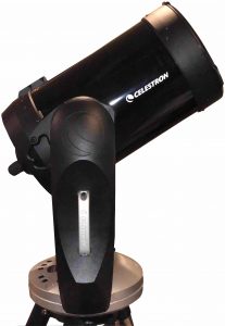 These forks rotate around the vertical or azimuth axis. The telescope is attached to the forks and can pivot on the horizontal or altitude axis. This system is obviously quite simple to construct and operate, but to track celestial objects, in their apparent circular paths across the sky, requires nearly constant adjustment of both axes. The introduction of microprocessor-based control systems has made this tracking viable.
Equatorial Mount
An equatorial mount has two perpendicular axes. The first axis is aligned with the earth’s axis of rotation, right ascension. The second is perpendicular to the first, declination. The telescope is attached to the second axis. To track a celestial object using this mount, the telescope is pointed to the desired object, found at a specific right ascension and declination, and then a constant sidereal clock drives the right ascension axis to compensate for the earth’s rotation.
Open Fork Mount
An alt-azimuth fork mount can be configured to benefit from the features 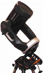 of an equatorial mount by aligning the azimuth axis with the earth’s axis of rotation, providing motion in right ascension. The telescope can then swing between the forks in declination. The device used to align the fork’s axis with that of the earth is commonly referred to as a wedge. With the addition of a wedge, the alt-azimuth mount must only be driven in right ascension to track celestial objects.
Field Rotation
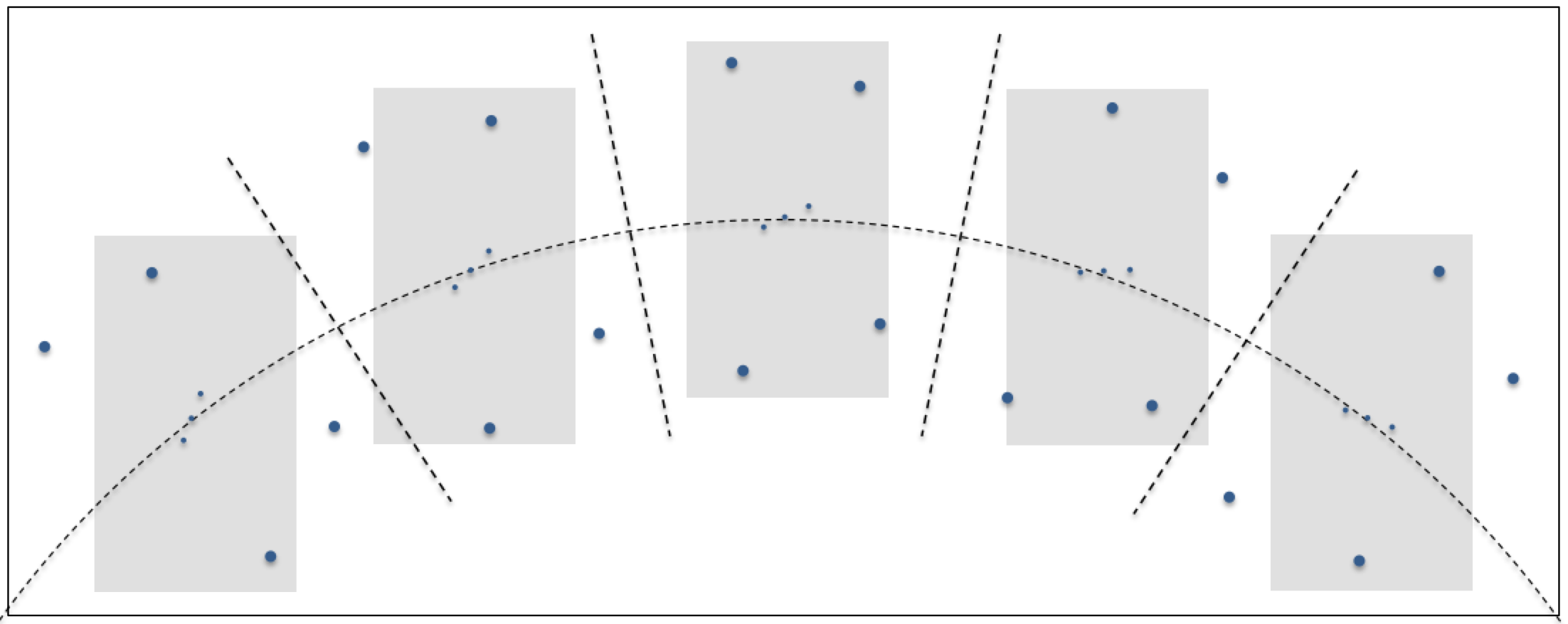
As a constellation rises, crosses the sky on an apparent circular arc and sets, you’ve likely noticed that it appears to rotate. For example, as the constellation Orion rises in the east it may appear to be leaning slightly to the left, at its highest altitude it may be upright and as it sets it appears to be leaning to the right. This is illustrated below.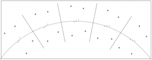 Let’s continue using the Orion constellation as our example. If you’re imaging with a system on an equatorial mount, the telescope and associated camera rotate in right ascension, as illustrated below. The gray rectangles in the figure represent the field of view of the imaging system. The camera retains its relative orientation to the celestial body being photographed. If the equatorial mount is accurately aligned with the earth’s axis, no field rotation occurs.
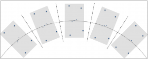
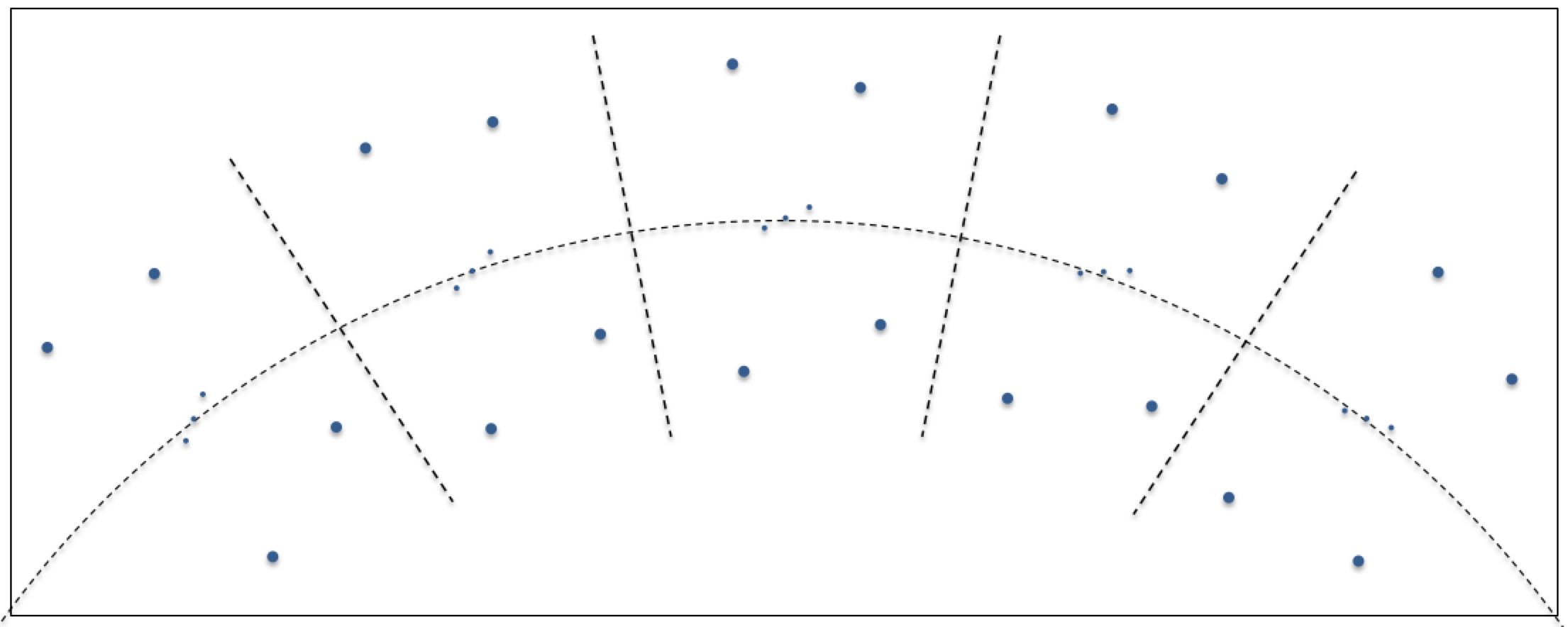
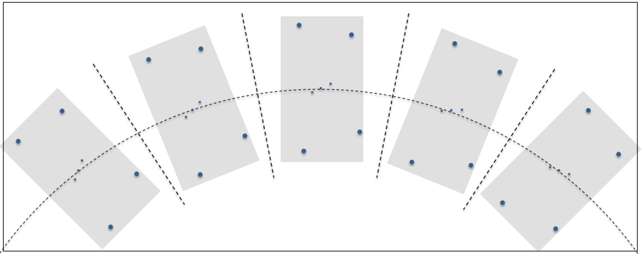
Unlike the previous example, if you’re imaging with a telescope on an alt-azimuth mount you will experience field rotation. In the following illustration, the gray rectangles again represent the field of view of the imaging system. Over time the imaging system remains centered on the middle star of Orion’s belt, but the camera remains level with the horizon due to the orientation of the mount’s two axes of rotation.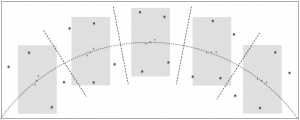
Notice in the above figure that Orion appears to rotate in the field of view as time passes. If the gray boxes represent distinct times within a long exposure, the stars in the constellation would appear as arcs rotating in a clockwise direction around the center of the frame, in this case, the middle star of Orion’s belt. This is what is meant by field rotation and it is generally undesirable.
It should be clear that equatorially mounted systems do not suffer from field rotation issues. However, this is only true if they are well aligned with the earth’s axis of rotation. While alt-azimuth mounted systems typically suffer from field rotation, solutions have been developed that rotate the imaging system to counter the field rotation. While some of these solutions have been available to amateur observers in the past, it doesn’t appear that any commercial solutions are currently available. In addition, software can be used during post processing of images to remove some of the artifacts introduced by field rotation.
The above examples illustrate the basic issues related to field rotation and astrophotography. However, field rotation is more complex than first meets the eye. In the northern hemisphere when looking south, like in our example above, the field rotation is in a clockwise direction. Looking north we observe counterclockwise field rotation, and this complexity is just the beginning. In the next section, we’ll investigate the math describing field rotation and present associated graphs.
The Math of Field Rotation
As eluded to in the previous section, field rotation is more complex than our simple examples lead one to believe. It would be easy to believe that the rate of rotation is constant or that rotation continues in the same direction as observed bodies fall below the horizon, neither are true. In this section, we’ll introduce the math behind field rotation and illustrate graphically what this means. The rate of field rotation is defined as,
![\[ \omega_f = \omega_{earth} \times \cos latitude_{observer} \times \frac{\cos azimuth}{\cos altitude} \]](https://kelly.flanagan.io/wp-content/ql-cache/quicklatex.com-d836948c54e0b3993f67548b7403732c_l3.png "Rendered by QuickLaTeX.com")
where  is the angular velocity of the field rotation in degrees per second,
  is the angular velocity of the earth’s rotation in degrees per second,
  is the latitude where the observations are made, and
  and
and  describe the coordinates of the celestial body of interest, at the time of observation, in degrees.
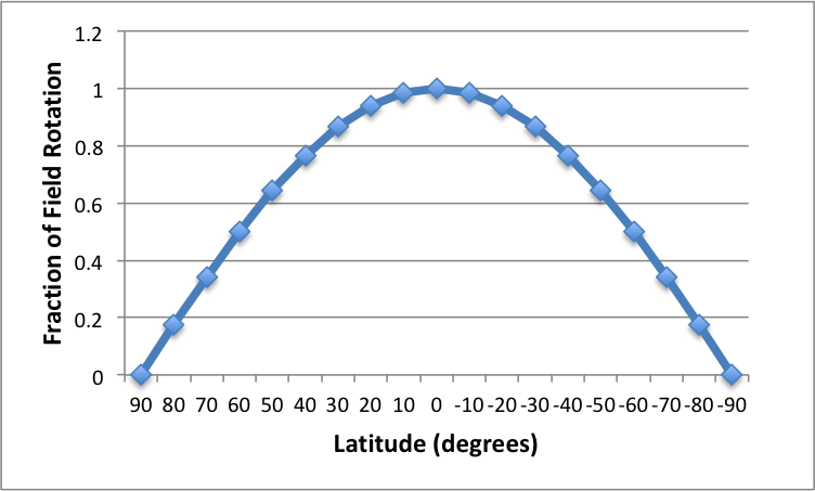
There are a few interesting observations regarding this equation. First, if the observer is at either pole, the  will be zero resulting in being zero. This is easily visualized if you imagine standing precisely on either pole and observing the movement of the stars. They will move around you with no change in altitude. This path is easily tracked by rotating around the azimuth axis of an alt-azimuth mount. Second, the field rotation is maximal at the equator where is equal to 1. However, as illustrated in the following figure, the increase in field rotation from latitude 40° north to the equator, for any given azimuth and altitude, is only about 30%. In this figure the horizontal axis is latitude in degrees, where negative values represent latitudes in the souther hemisphere. The vertical axis is the value of .
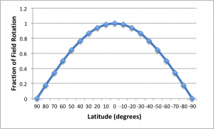
Second, if the  is zero we have a divide by zero issue. This occurs at an altitude of 90°, the zenith, where field rotation is infinite and cannot be tracked by an alt-azimuth mounted telescope.
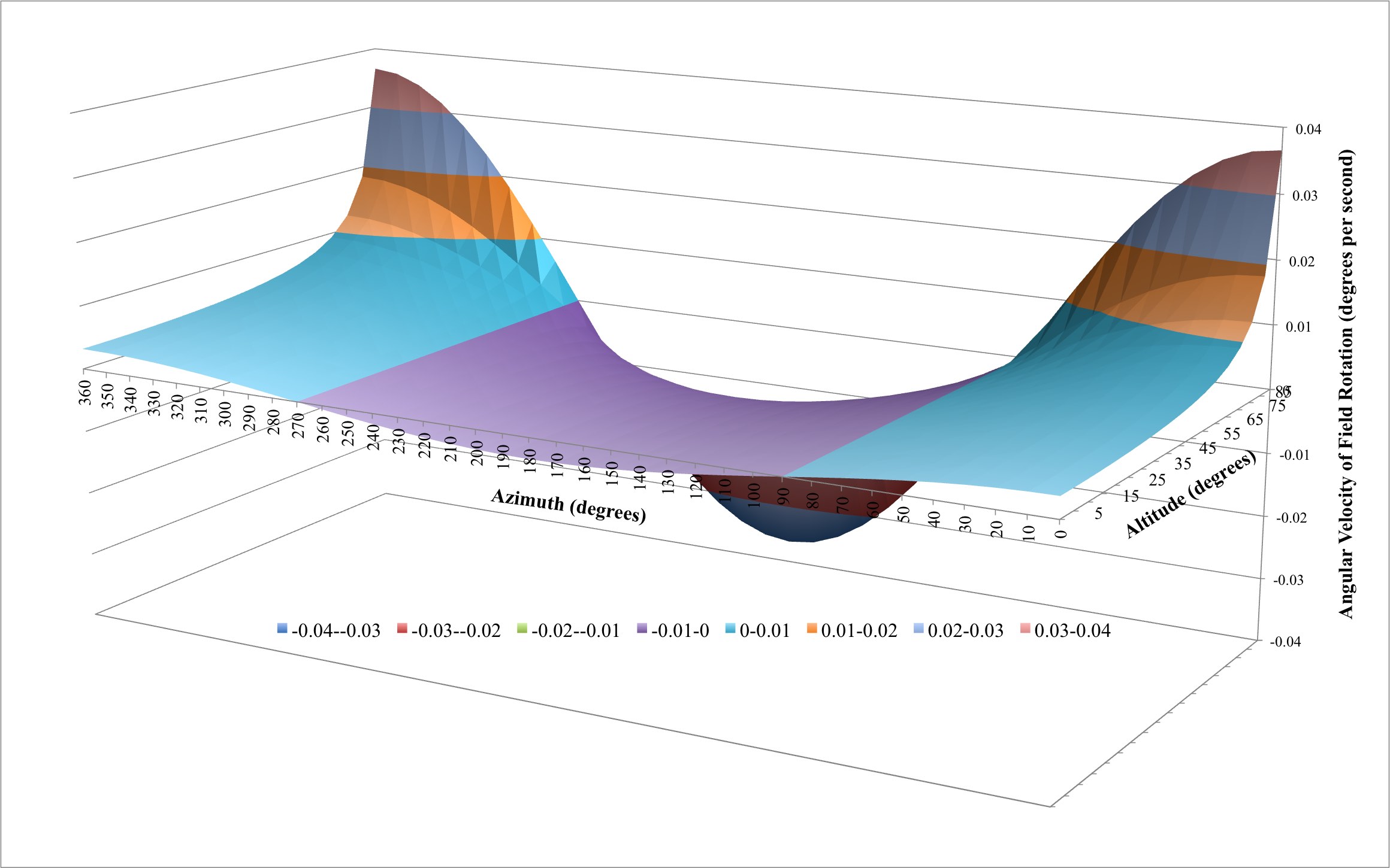
With regard to the field rotation equation, there are four variables of interest, namely , , and . Four dimensions are difficult to visualize so we’ll use my latitude of 40.3245° north and analyze the other three variables graphically.
The vertical axis of the above surface plot illustrates the angular velocity of the field rotation, in degrees per second, for various values of azimuth (horizontal axis) and altitude (depth axis). There are several interesting insights worth pointing out. First, at altitudes less than 65° the field rotation never exceeds 0.01° per second regardless of the azimuth chosen. Second, the field rotation never exceeds 0.01° per second for altitudes up to 75° for azimuths between 240° and 300° and 60° and 120°. In other words, looking due east or due west is far better than looking north or south. Finally, looking north or south results in high rates of rotation.
This section has illustrated the mathematical theory governing field rotation. While the math is fairly straightforward, the results are more complicated than one may have initially thought. In the next section, we’ll determine the impact field rotation has on astrophotography for our specific system and reexamine the surface plot above in terms of safe and ill-advised zones for various exposure lengths.
Impact on Astrophotography
For long exposures using imaging systems attached to alt-azimuth or poorly aligned equatorial mounts, field rotation is an issue that degrades image quality. In the previous section, we presented an approach to determine the angular velocity of the field rotation for a given latitude, azimuth and altitude. In this section, we’ll use that information to quantitatively determine how field rotation impacts image quality using systems with various characteristics.
Acceptable Field Rotation
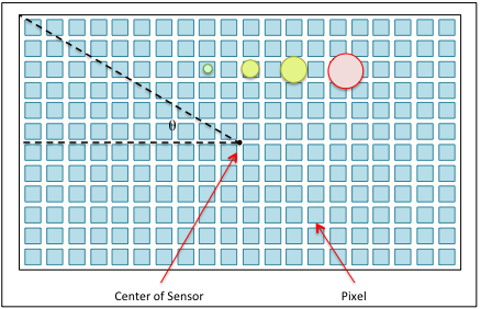
Imaging system characteristics such as focal length, aperture, f-number, exposure length, sensor size and pixel size play important roles in astrophotography. The characteristics that determine the level of impact field rotation has on image quality are focal length, the size of the sensor and the associated pixels. The following figure is a representation of an image sensor made up of a two-dimensional array of pixels. The green, 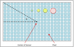 yellow and red disks represent seeing disks projected onto the sensor with angular sizes of 1″, 2″, 3″ and 4″ respectively. This is to scale for a sensor with a pixel size of 4.78µm and a system focal length of 560mm. The sizes of these disks are proportional to the focal length of the system as described below.
![\[ Size_{disk} = \frac{2\pi}{360°} \theta_{disk} \times Focal\;Length \]](https://kelly.flanagan.io/wp-content/ql-cache/quicklatex.com-2efa9da6dad74b28418f84310f90a2cf_l3.png "Rendered by QuickLaTeX.com")
where  is the size of the seeing disk on the sensor in meters,
  is the angular size of the seeing disk in degrees and
  is the focal length of the optical system in meters. The four seeing disks illustrated on the sensor are approximately 2.71µm, 5.43µm, 8.14µm and 10.86µm in diameter.
While an image is being exposed, the field is rotating at an angular velocity . For a specific exposure time,  , the angle of image rotation
  can be computed as
  . While all objects in the field of view rotate around the center at the same angular velocity, those furthest from the center cover more distance. To ensure good image quality, the distance travelled must be less than a few pixels on the sensor. In the next section, we’ll try and quantify how much image rotation can be tolerated while still achieving esthetically pleasing results.
The Rule of 500
To determine just how many pixels can be traversed without significant impact, we’ll turn to the rule of 500 used by photographers to image the night sky. It should be noted that this rule was not developed to deal with field rotation, but rather to deal with star movement relative to a stationary camera. However, it does suggest the amount of movement that can be tolerated and still yield pleasing results. This rule of thumb suggests that the maximum length of an exposure, without significant star trails, is computed by dividing 500 by the focal length of the system measured in mm. The angular distance a star image travels across the sensor in this length of time is derived below.
![\[ \theta_{star} = \omega_{earth} \times time_{exposure} \]](https://kelly.flanagan.io/wp-content/ql-cache/quicklatex.com-fcac9fdf8a629a850cdbd850b7e51c72_l3.png "Rendered by QuickLaTeX.com")
where  is the angular distance in degrees traveled by a star in measured in seconds given that the earth is rotating at the angular velocity of measured in degrees per second.
According to the rule of 500 an appropriate exposure time is 500 divided by the focal length of the optical system measured in mm,
![\[ \theta_{star} = \omega_{earth} \times \frac{500}{Focal\;Length} \]](https://kelly.flanagan.io/wp-content/ql-cache/quicklatex.com-f0bf4e75ee3afbf98349b17ce13185fe_l3.png "Rendered by QuickLaTeX.com")
or
![\[ \theta_{star} = \frac{\omega_{earth}}{2 \times Focal\;Length} \]](https://kelly.flanagan.io/wp-content/ql-cache/quicklatex.com-db2a1b177083f74734251f02994d42bf_l3.png "Rendered by QuickLaTeX.com")
where is now measured in meters. By determining the fraction of the sensor that represents and multiplying it by the number of pixels, we’ll get the number of pixels traversed when applying the rule of 500. To start with we know that,
![\[ FOV = \frac{360°}{2\pi} \frac{Sensor\;Size}{Focal\;Length} \]](https://kelly.flanagan.io/wp-content/ql-cache/quicklatex.com-b85924f130beef0d32e0213bdf7d9e5e_l3.png "Rendered by QuickLaTeX.com")
and
![\[ Pixel\;Count = \frac{Sensor\;Size}{Pixel\;Size} \]](https://kelly.flanagan.io/wp-content/ql-cache/quicklatex.com-e24a2e0a8bdfb832b5d20921a4f66c62_l3.png "Rendered by QuickLaTeX.com")
where  is the field of view projected onto the sensor measured in degrees,
  is the size of the sensor in a particular dimension measured in meters, is the focal length of the system measured in meters,
  is the number of pixels in the same dimension as mentioned above and
  is the size of one pixel, measured in meters.
Dividing by and multiplying by  we obtain,
![\[ \frac{\theta_{star}}{FOV} \times \frac{Sensor\;Size}{Pixel\;Size} = \frac{\frac{\omega_{earth}}{2 \times Focal\;Length}}{\frac{360°}{2\pi}\frac{Sensor\;Size}{Focal\;Length}} \times \frac{Sensor\;Size}{Pixel\;Size} \]](https://kelly.flanagan.io/wp-content/ql-cache/quicklatex.com-927ee2791aca7bc9f5d14681259039cd_l3.png "Rendered by QuickLaTeX.com")
Simplifying we obtain,
![\[ \frac{\theta_{star}}{FOV} \times \frac{Sensor\;Size}{Pixel\;Size} = \frac{\pi}{360°}\frac{\omega_{earth}}{Pixel\;Size} \]](https://kelly.flanagan.io/wp-content/ql-cache/quicklatex.com-47ad142e5189d9e80784cdaaa9528b9f_l3.png "Rendered by QuickLaTeX.com")
Finally, we recognize that  is simply the number of pixels traversed by the seeing disk on the sensor, resulting in
![\[ Pixels_{traversed} =\frac{\pi}{360°}\frac{\omega_{earth}}{Pixel\;Size} \]](https://kelly.flanagan.io/wp-content/ql-cache/quicklatex.com-4633060f75646fd010d8e456fc3de1ff_l3.png "Rendered by QuickLaTeX.com")
where  are the number of pixels that can be traversed without leaving significant star trails according to the rule of 500, is the rotational velocity of the earth in degrees per second and is the size of each pixel in meters.
A sidereal day is 23 hours 56 minutes and 4.1 seconds or 86,164.1 seconds long. The earth rotates through 360° in this length of time resulting in being approximately equal to 0.00418° per second.
For a pixel size of 4.78µm, the rule of 500 suggests that 7.63 pixels can be traversed. We’ll round down to ensure better image quality. For the remainder of this work we’ll assume that if a seeing disk traverses 7 or fewer pixels across the sensor, due to field rotation, the image quality will be acceptable.
It is important to keep in mind that the rule of 500 has nothing to do with field rotation. However, photographers have used this rule to achieve good results shooting the night sky without significant star trails in their photographs. If stars traversing 7 pixels in these photographs are not objectionable, they shouldn’t be in our images either.
Acceptable Viewing
In the previous section we determined that star images traversing 7 or fewer pixels across the sensor would be acceptable. In this section we’ll investigate what impact we can expect due to field rotation and determine where in the night sky it is safe to image without having elongated stars in our photographs.
Given a rectangular image sensor, the distance an object travels in terms of rotational velocity and distance from the center of the sensor is described by,
![\[ D = \frac{2 \pi R}{360} \times \omega_f \times time_{exposure} \]](https://kelly.flanagan.io/wp-content/ql-cache/quicklatex.com-8788879548b4f4c2ac9eecba4a368225_l3.png "Rendered by QuickLaTeX.com")
where  is the distance in meters an object travels across the sensor at a distance
  from the center of the sensor, is the distance from the center of the sensor to the object of interest in meters, is the field rotational velocity in degrees per second and is the length of the exposure in seconds. Combining our initial equations for with this equation we have,
![\[ D = \frac{2 \pi R}{360} \omega_{earth} \times \cos latitude_{observer} \times \frac{\cos azimuth}{\cos altitude} \times time_{exposure} \]](https://kelly.flanagan.io/wp-content/ql-cache/quicklatex.com-3d060f80dfec6183466f1f60eb9a1a3b_l3.png "Rendered by QuickLaTeX.com")
where is the distance an object travels across the sensor in meters, is the distance from the center of the sensor to the object of interest in meters, is the angular velocity of the earth’s rotation in degrees per second, is the latitude where the observations are made, and describe the coordinates of the celestial body of interest in degrees and is the length of the exposure in seconds.
Let’s consider the characteristics of a specific CMOS sensor, the IMX071. This sensor is 23.6mm x 15.6mm with a 28.4mm diagonal. The pixel size of this sensor is 4.78µm and they are organized in a two-dimensional array that measures 4944 x 3284 pixels. While objects at the extreme corners of the sensor are not captured as they rotate through the field, their distance from the center is a good worst case measure since they travel further than anything else in the field for any given .
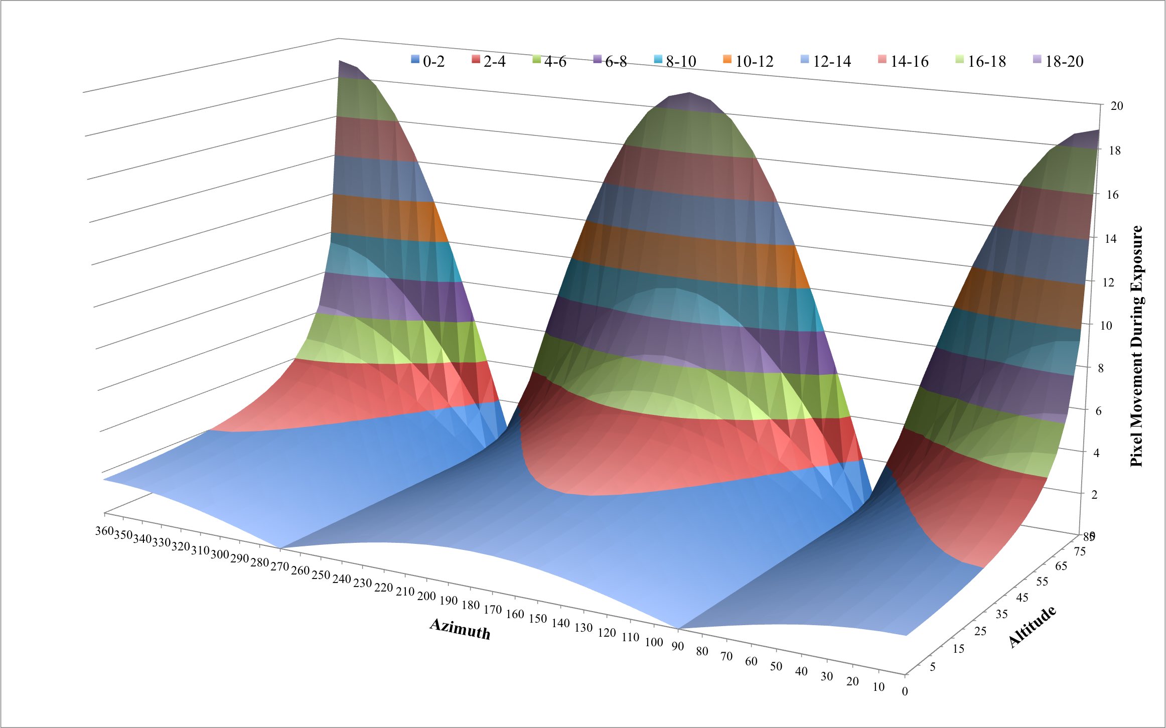
If we assume the same of 40.3245° north as before and an exposure time of 10 seconds, we obtain the surface below. 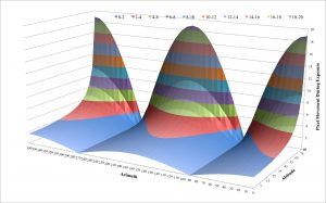 The vertical axis is the number of pixels traversed during a 10 second exposure, the other two axes represent the azimuth and altitude of the observed object.
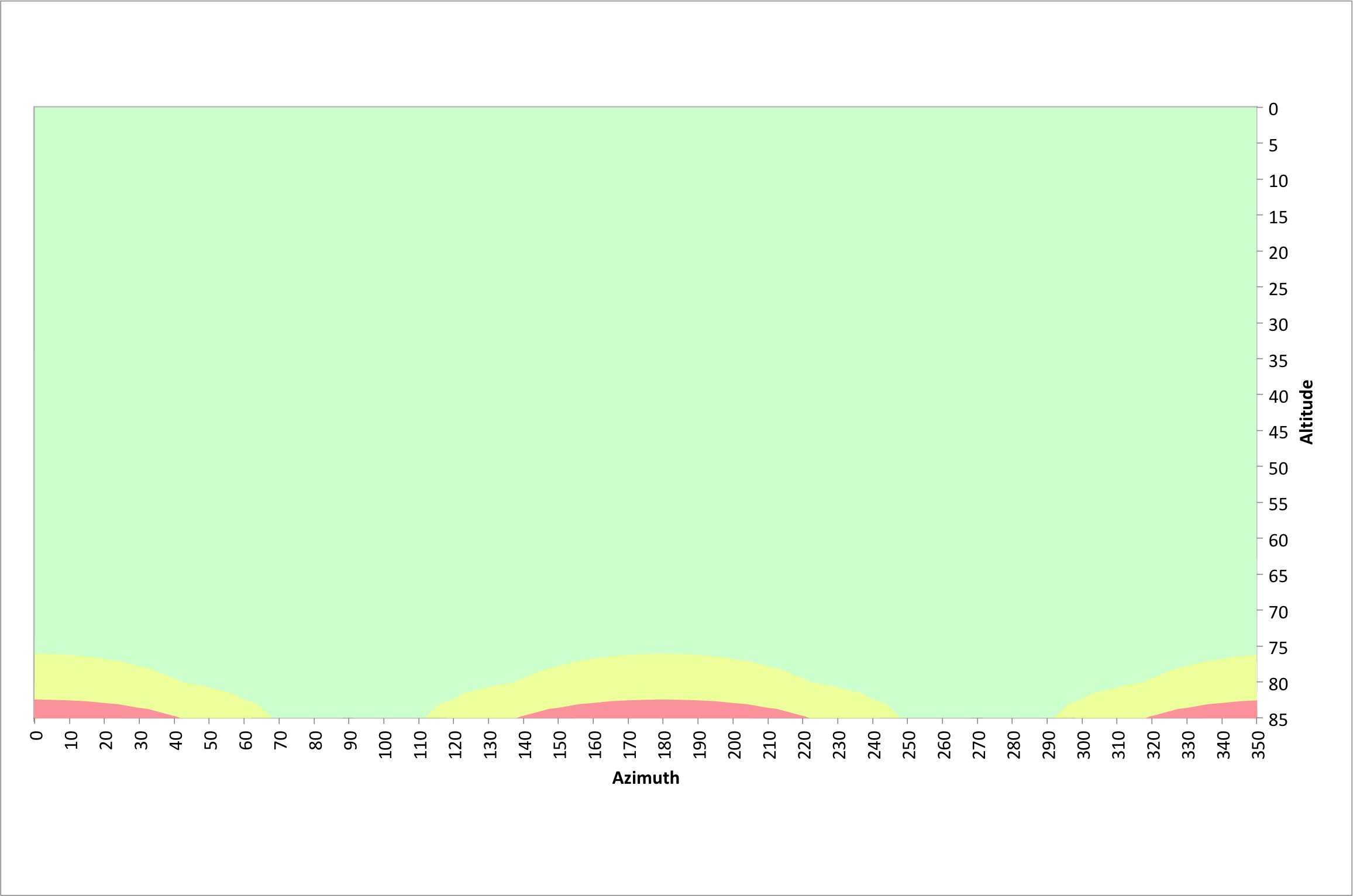
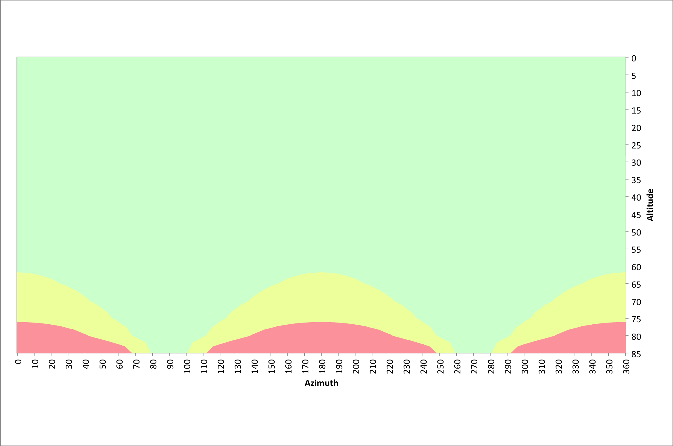
For good image quality it is important to have as little movement as possible, but less than 7 pixels according to the rule of 500 discussed in the previous section. The following figure illustrates azimuths and altitudes that result in good 10 second exposures at a latitude of 40.3245° north.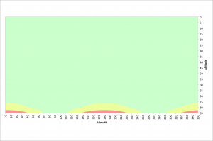
The green area illustrates where pixel traversals of 7 pixels or less occur. The yellow areas have pixel traversals of 7 to 14 pixels and the red regions represent pixel traversals greater than 14 pixels.
For altitudes less than 75°, acceptable images can be acquired at any azimuth value. Between 70° and 110° azimuth and 250° and 290° azimuth, acceptable images can be obtained at altitudes up to 85°. There are few restrictions for 10 second exposures. Also recall that these values are based on the very corner of the sensor where field rotation has the biggest impact.
The next two figures illustrate azimuths and altitudes that result in good 20 and 30 second exposures at a latitude of 40.3245° north.
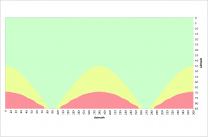
Exposure times of 30 seconds result in far more restrictions. The poles should be avoided above 45° and only due east and west are virtually unrestricted.
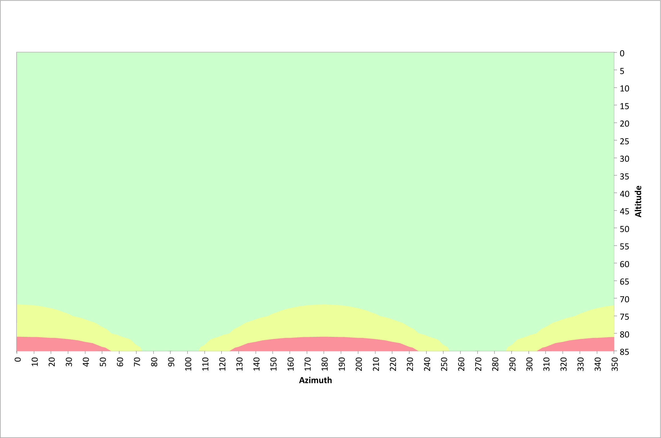
As stated earlier, there is no field rotation at the poles of the earth. The equatorial region suffers the most field rotation. The following figure illustrates azimuths and altitudes that result in good 10 second exposures at the equator, latitude 0°.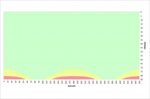 As previously stated, moving from a latitude of ~40° to 0° has little impact on the effects of field rotation. There are no restrictions below 70° of altitude and almost no restrictions in the vicinity of due east and due west.
In this section we discussed and visualized the impact of field rotation on astrophotography and discussed where in the sky it is acceptable to image. In the next section we’ll discuss these results as they apply to a specific use case.
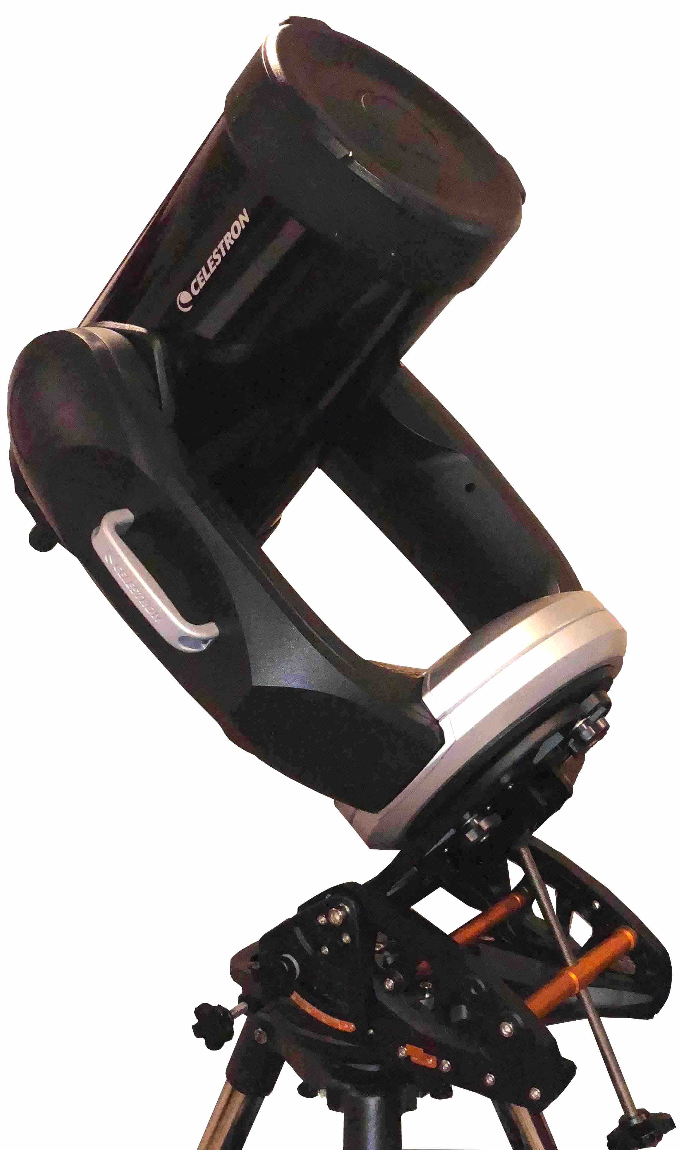
Celestron CPC 1100 GPS XLT
In the previous sections we have described field rotation and determined its impact on astrophotography in terms of azimuth, altitude, latitude and exposure time. In addition, we have hypothesized, using the rule of 500, that star images can cross 7 or fewer pixels on the image sensor without significantly degrading image quality. In this section, we’ll investigate how this impacts images captured using a Celestron CPC 1100 GPS XLT telescope on an alt-azimuth mount. Finally, we’ll determine under what circumstances this configuration can successfully capture images of deep space objects (DSO).
Specific Configuration
The system of interest is a Celestron CPC 1100 Schmidt-Cassegrain telescope mounted in its standard alt-azimuth mount. The system includes a Hyperstar 3 lens system and a ZWO ASI071MC Pro camera. The Hyperstar system replaces the secondary mirror of the telescope and results in an optically fast f/2 system with a focal length of 560mm.
The ZWO ASI071MC Pro camera uses the IMX071 sensor that measures 23.6mm x 15.6mm with a 28.4mm diagonal. The pixel size of this sensor is 4.78µm and they are organized in a two-dimensional array that measures 4944 x 3284 pixels.
Astrophotography Limitations
An f/2 optical system is quite fast, which allows shorter exposure times than used by astrophotographers using more traditional f5.6 or slower refractor telescope systems. In fact, an f/2 system is 8 times faster than an f/5.6 system. While there is much debate around the optimal exposure time of sub-exposures used in stacking, there are many who use 2 to 5 minute sub-exposure times with f/5.6 systems. Compared to an f/5.6 system, an f/2 system can collect the equivalent amount of light in 15 to 37.5 seconds.
Given my latitude of 40.3245° north, our use of the rule of 500 and the above information we can once again refer to the following figure. Again, the green area of this figure is where the field rotation results in fewer than 7 pixels being traversed at the corner of the sensor during a 30 second exposure. The yellow and red regions violate the rule of 500 for this long of an exposure.
On our f/2 system a 30 second exposure is equivalent to a 4 minute exposure on an f/5.6 system. This should be satisfactory for sub-exposure times for many DSOs. The green area in the above figure represents azimuths and altitudes where we can expect good results. We should have good results anywhere below an altitude of 45°. Since seeing is generally not ideal below an altitude of 30°, we should expect to find success at any azimuth between an altitude of 30° and 45°. We can also find success at azimuths from 55° to 125° and 235° to 305° for altitudes up to 65°. Due east and west we have virtually no limitations.
While the exposure times discussed above result in acceptable field rotation within a give sub-exposure, there will be significant field rotation over the set of sub-exposures that will be stacked during post processing. Removing this field rotation requires the stacking algorithm to align stars using both translation and rotation. Nebulosity 4 can perform star alignment using translation, rotation and scaling. I’m confident other tools can as well.
Summary
Alt-azimuth mounted telescopes used for astrophotography suffer from field rotation. Field rotation causes star images on the sensor to circle around the center of the field of view. To achieve acceptable results the amount of movement must be minimized. The rule of 500 suggests that if 7 or fewer pixels are traversed during an exposure, the outcome in terms of star trails will be acceptable. For 10 second exposures, there are few limitations on where in the sky an object can be photographed. As the exposure times increase to 30 seconds far more restrictions exist, but success can be found.
Several obvious things can be done to improve the likelihood of acquiring acceptable results. First, imaging where field rotation will result in 7 or fewer pixel traversals will help. These areas are identified in the previous graphs. Second, the shorter the exposure times the better. While 30 second exposures have a few unacceptable areas of the sky, 10 second exposures have virtually no limitations. Finally, since field rotation issues decrease as you move towards the center of the sensor, cropping acquired images will help.
For our Celestron CPC 1100 GPS XLT at ~40° north latitude operating in an f/2 configuration, there are few limitations when taking 10 second exposures. Since f/2 is 8 times faster than a typical f/5.6 refractor telescope used for astrophotography, 30 second exposures, or even shorter, will likely result in acceptable sub-exposures. Now it is time to collect data and see how accurate these findings are.
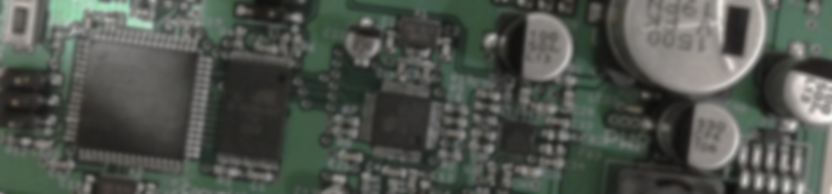
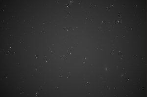 The figure to the right is one of the 110 sub-exposures. The most significant visual issue is the significant vignetting. In addition, these exposures are likely too long given the conditions. Future attempts will be made with more subs, but shorter exposure times.
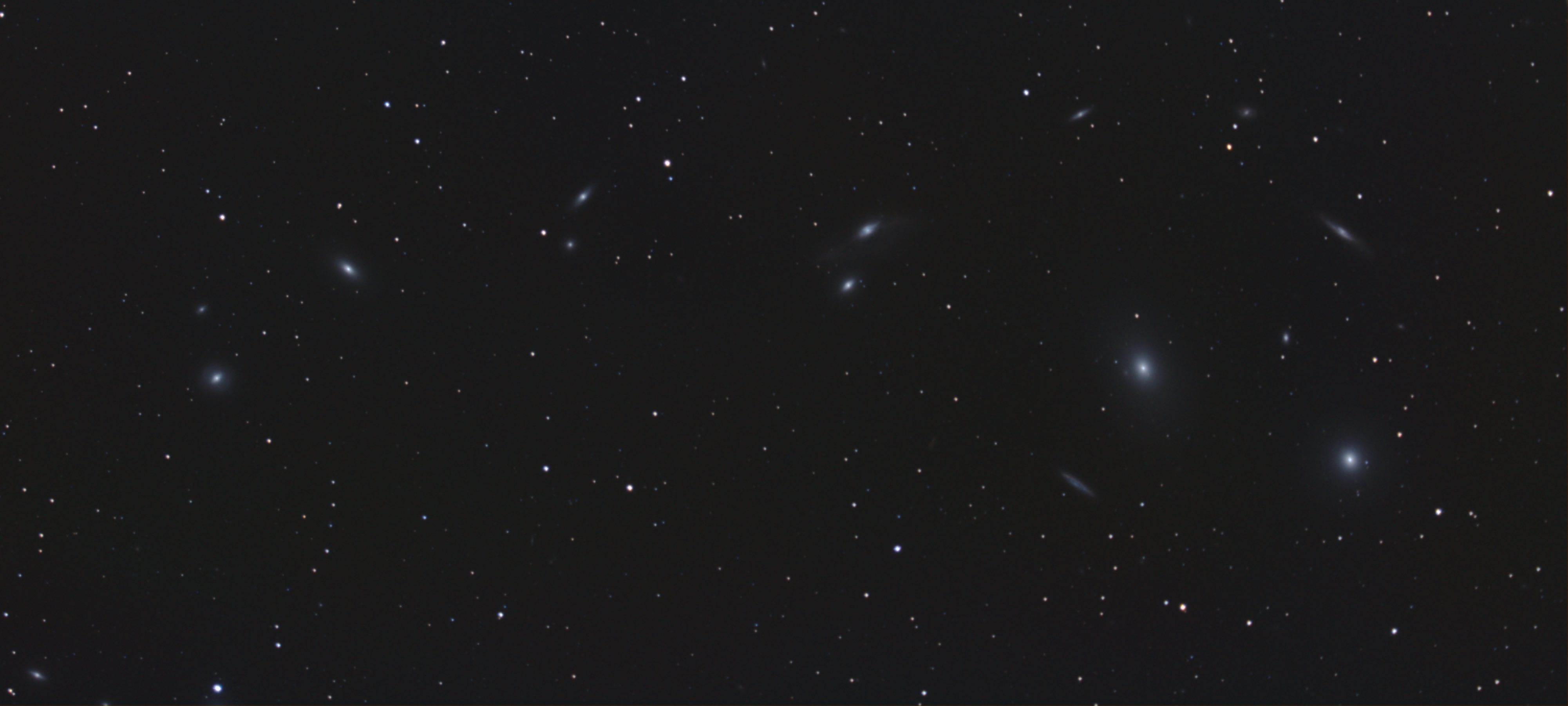
 acquired with a 5 second exposure time with a camera gain of 200 and an offset of 50. The figure to the right is one of the 120 sub-exposures. The most significant visual issue is again the significant vignetting. In addition, there is significant noise due to the high gain used. In the future, I am unlikely to use gains greater than unity.
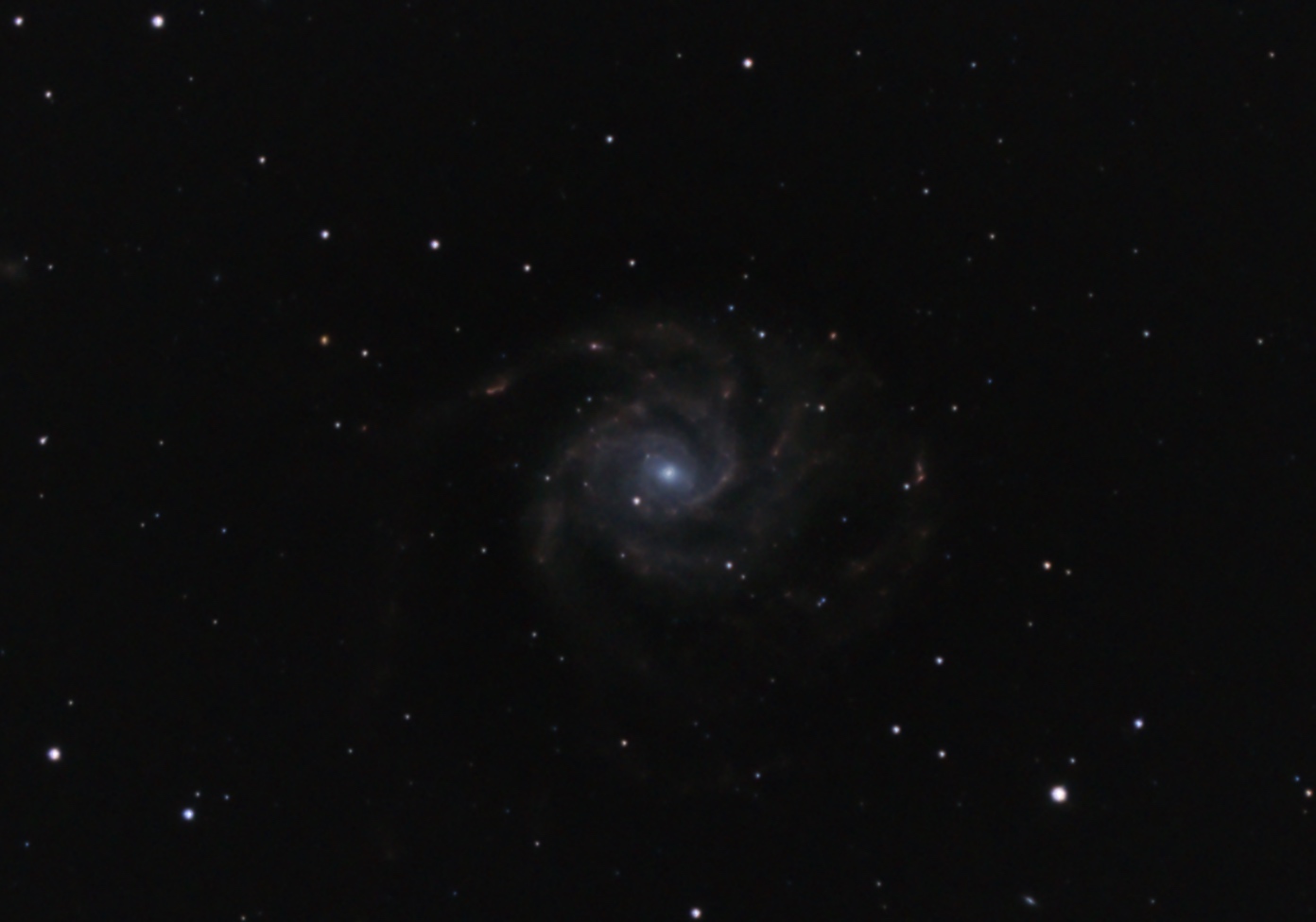
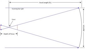
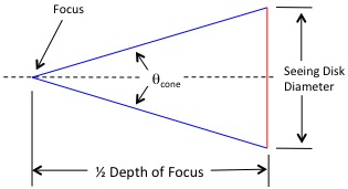
 , formed by the sides of the cone at the focus, is
![\[ \theta_{cone} = 2 \sin^{-1}(\frac{\text{Aperture}}{2 \times \text{Focal Length}}) \]](https://kelly.flanagan.io/wp-content/ql-cache/quicklatex.com-85d735a47c5f110e194d149af7651594_l3.png "Rendered by QuickLaTeX.com")
![\[ \theta_{cone} = 2 \sin^{-1}(\frac{1}{2 \times \text{f-number}}) \]](https://kelly.flanagan.io/wp-content/ql-cache/quicklatex.com-13fd8754f1ea9cf8df047752e06e5edd_l3.png "Rendered by QuickLaTeX.com")
![\[ \frac{1}{2}F_{depth} = \frac{\frac{1}{2}D_{size}}{\tan \frac{\theta_{cone}}{2}} \]](https://kelly.flanagan.io/wp-content/ql-cache/quicklatex.com-2d2b84fb2adf3cbbd7f7ab57f7622bcf_l3.png "Rendered by QuickLaTeX.com")
![\[ F_{depth} = \frac{D_{size}}{\tan \frac{\theta_{cone}}{2}} \]](https://kelly.flanagan.io/wp-content/ql-cache/quicklatex.com-549cddc5792752303d492b1060d12daf_l3.png "Rendered by QuickLaTeX.com")
 is the depth of focus in meters,
  is the size of the seeing disk in meters and
 ![\[ D_{size} = \frac{2\pi}{360} \theta_{disk} \times \text{Focal Length} \]](https://kelly.flanagan.io/wp-content/ql-cache/quicklatex.com-c302c8c71436791e9a6a170001895e9b_l3.png "Rendered by QuickLaTeX.com")
![\[ F_{depth} = \frac{\frac{2\pi}{360} \theta_{disk} \times \text{Focal Length}}{\tan (\sin^{-1}(\frac{1}{2 \times \text{f-number}}))} \]](https://kelly.flanagan.io/wp-content/ql-cache/quicklatex.com-8cf1ec36769c7d1995a547eaa3cd729d_l3.png "Rendered by QuickLaTeX.com")
![\[ F_{depth} = \frac{\frac{2\pi}{360} \theta_{disk} \times \text{Focal Length}}{\frac{(\frac{1}{2 \times \text{f-number}})}{\sqrt{1-(\frac{1}{2 \times \text{f-number}})^2}}} \]](https://kelly.flanagan.io/wp-content/ql-cache/quicklatex.com-66b4759faa00c2a1c621ddf7c3157231_l3.png "Rendered by QuickLaTeX.com")
 the above equation can be simplified.
![\[ F_{depth} = \frac{\frac{2\pi}{360} \theta_{disk} \times \text{Focal Length}}{\frac{1}{2 \times \text{f-number}}} \]](https://kelly.flanagan.io/wp-content/ql-cache/quicklatex.com-db6e2a02a6536969f0b1f49311b60b9c_l3.png "Rendered by QuickLaTeX.com")
![\[ F_{depth} = \frac{4\pi}{360} \frac{\theta_{disk}}{3600} \times \frac{(\text{Focal Length})^2}{\text{Aperture}} \]](https://kelly.flanagan.io/wp-content/ql-cache/quicklatex.com-496667bdecdb69699cddca98d329544c_l3.png "Rendered by QuickLaTeX.com")
![\[ \theta = 1.22\times\frac{\lambda}{d} \]](https://kelly.flanagan.io/wp-content/ql-cache/quicklatex.com-7cea4e6b8b980f492a18c35cde617c0b_l3.png "Rendered by QuickLaTeX.com")


![\[ \theta = \frac{360}{2\pi} \times 3600 \times 2.44\times\frac{\lambda}{d} \]](https://kelly.flanagan.io/wp-content/ql-cache/quicklatex.com-0ec98cb1c544e75f2d57e571ffaad049_l3.png "Rendered by QuickLaTeX.com")
![\[ F_{depth} = \frac{4\pi}{360} \frac{\frac{360}{2\pi} \times 3600 \times 2.44\times\frac{\lambda}{d}}{3600} \times \frac{(\text{Focal Length})^2}{\text{Aperture}} \]](https://kelly.flanagan.io/wp-content/ql-cache/quicklatex.com-71e7aedd226e9361ff2943c840814fbb_l3.png "Rendered by QuickLaTeX.com")
![\[ F_{depth} = 2 \times 2.44\times\frac{\lambda}{d} \times \frac{(\text{Focal Length})^2}{\text{Aperture}} \]](https://kelly.flanagan.io/wp-content/ql-cache/quicklatex.com-d7ad27994d194babb7e13469fd65e3a3_l3.png "Rendered by QuickLaTeX.com")
![\[ F_{depth} = 4.88 \times \lambda \times \text{f-number}^2 \]](https://kelly.flanagan.io/wp-content/ql-cache/quicklatex.com-ae70cf5a51b2b2f7572aedfb3fcea197_l3.png "Rendered by QuickLaTeX.com")


![\sqrt[5]{100}](https://kelly.flanagan.io/wp-content/ql-cache/quicklatex.com-1728cbd7eaa27632e03267ed0b354ead_l3.png "Rendered by QuickLaTeX.com")
![\[ FOV = \frac{Sensor\;Size}{Focal\;Length} \]](https://kelly.flanagan.io/wp-content/ql-cache/quicklatex.com-2240024c3e54b24d119d839881f3e6a2_l3.png "Rendered by QuickLaTeX.com")

![\[ FOV_{pixel} = \frac{\frac{Sensor\;Size}{Pixel\;Count}}{Focal\;Length} \]](https://kelly.flanagan.io/wp-content/ql-cache/quicklatex.com-7b100b4f02dc7b0a3a37612cb0af671e_l3.png "Rendered by QuickLaTeX.com")
![\[ FOV_{pixel} = \frac{Pixel\;Size}{Focal\;Length} \]](https://kelly.flanagan.io/wp-content/ql-cache/quicklatex.com-065924f2d1892fdd12cc82858179d4cc_l3.png "Rendered by QuickLaTeX.com")
![\[ 1.22\times\frac{\lambda}{d} = \frac{Pixel\;Size}{Focal\;Length} \]](https://kelly.flanagan.io/wp-content/ql-cache/quicklatex.com-48e56711238a6d91f3705bef43e78467_l3.png "Rendered by QuickLaTeX.com")

![\[ Pixel\;Size = 1.22\times \lambda \times \text{f-number} \]](https://kelly.flanagan.io/wp-content/ql-cache/quicklatex.com-b6728bf76bd57e9cd4beffdfa73660ba_l3.png "Rendered by QuickLaTeX.com")