Introduction

There are numerous issues to consider when choosing a camera for astrophotography. Consideration must be given to the type of astrophotography of interest, the specifications of the chosen telescope, and the camera style, technology and sensor specifications. This document addresses these issues in general terms and illustrates specifics based on an example telescope, a Celestron CPC 1100 GPS XLT.

Objects of Interest

The two types of astrophotography investigated in this document are planetary imaging and deep space object (DSO) photography. Planets and DSOs have unique characteristics that demand different approaches for capturing aesthetically pleasing images. The two characteristics that most influence the employed methodologies are apparent size and brightness.

The apparent size of celestial objects are measured in arc-seconds. The celestial sphere, like a circle, has an angular circumference of 360°, read as 360 degrees. Each degree can be subdivided into 60’, read as 60 arc-minutes, and each arc-minute can be subdivided into 60”, read as 60 arc-seconds. For reference the apparent size of our sun and moon are approximately 32’ or 1920”. The planets range in apparent size from Neptune at 2.21” up to Jupiter at 40.95”. In comparison DSOs in the Messier Catalog range in apparent size from M40 at 48” up to M31 at 10,680” or 178’.

The apparent brightness of celestial objects are measured in magnitude (m) as observed from earth. The brightness of an object can be measured in various wavelengths of the electromagnetic spectrum. We’ll restrict our interest to the visible spectrum where magnitudes are denoted m_v. Brighter objects have lower magnitudes, it’s an inverse relationship. The brightest object in the sky is the sun at magnitude -27 or m_v = -27. The magnitude scale is logarithmic. A difference in magnitude of 1 is equivalent to a change in brightness by a factor of  or approximately 2.512. The magnitudes of the planets range from Neptune at m_v = 7.96 up to that of Venus at m_v = -3.86. However, the most imaged planets range in brightness from Mars at m_v = 0.56 up to Venus at m_v = -3.86. In comparison the DSOs in the Messier Catalog range in magnitude from M91 at m_v = 10.2 up to M45 at m_v = 1.6. However the second brightest item in the Messier Catalog is M7 at m_v = 3.3, illustrating that M45 is a bright exception.

With regard to astrophotography, the planets are very small and relatively bright objects, while DSOs are huge in comparison and very dim. These differences lead to different imaging strategies which in turn influence equipment configuration and technology choices.

Telescopes

There are many types and sizes of telescopes. This document will not attempt to describe the various types or their strengths and weaknesses. Instead, it will cover basic configuration parameters that impact the imaging of planets and DSOs. From the previous discussion it should be clear that a large field of view is important for imaging DSOs and high magnification is essential for photographing the planets. These are competing requirements in terms of telescope specifications.

The aperture of a telescope is the width of the primary mirror or lens. Larger apertures are capable of resolving finer detail and collecting more light, resulting in lower exposure times. The focal length is the distance from the primary mirror or lens to where the image is focused. Longer focal lengths result in more magnification and narrower fields of view. The f-number, or speed of the telescope, is determined by dividing the focal length by the aperture. For a given aperture, planetary imaging demands a large f-number where high magnification is obtained. For imaging DSOs a low f-number yields less magnification and a greater field of view.

Astrophotographers acquire telescopes with as much aperture as they can afford and physically handle. Those photographing DSOs tend to acquire moderately sized apochromatic (APO) refractor based telescopes with f-numbers in the f/5.6 to f/7 range. They often add a focal reducer to further decrease the effective f-number. Those photographing planets tend to acquire telescopes with longer focal lengths and employ Barlow lenses to increase the focal length by a factor of 2, 3 and even 5.

Telescopes like the Celestron CPC 1100 GPS XLT have a large 280mm aperture. The Schmidt-Cassegrain telescope (SCT) design results in a focal length of 2800mm and an f-number of f/10. This configuration results in a narrow field of view and relatively long exposure times for faint DSOs. The addition of a Barlow lens to this configuration results in a system that is ideal for planetary imaging. Fortunately, Celestron included a removable secondary mirror to the CPC 1100 system that can be replaced by a lens system called Fastar or Hyperstar. These systems convert the telescope from a relatively slow f/10 system to a fast f/2 imaging system. In this configuration the CPC 1100 has a focal length of 560mm and a huge field of view of just over 2.76°. This convertible feature makes the CPC 1100 useful for both planetary and DSO imaging.

Cameras

There are many choices to be made when selecting a camera for astrophotography. These choices include the camera form factor, the sensor technology and detailed specifications such as sensor size, pixel depth and pixel size.

Camera Form Factors

While there are commercially available cameras specifically deigned for astrophotography, many photographers use modified DSLR cameras. The beneficial modification entails removing the infrared filter that sits permanently over the sensor of the camera. This renders the camera less than useful for regular photography, but allows the camera to be more sensitive to the wavelength of light produced by Hydrogen-alpha emission nebulae. These cameras may be used with nearly any telescope, but when placed in front of the optical path, using a system like Fastar or Hyperstar, the size and shape of the camera may block an unacceptable amount of light and introduce diffraction artifacts in captured images.

Many dedicated astrophotography cameras have better form factors that permit them to be connected within the optical path without negatively impacting the amount of light entering the system. In addition, many of these cameras are cooled, reducing sensor noise and increasing the quality of the finished results. However, these cameras have connected cables that introduce unwanted diffraction patterns in images.

Sensor Technology – CCD or CMOS

Commercially available astrophotography cameras are available with CCD and CMOS sensors. CCD sensors have an edge over CMOS sensors in image quality, but CCD sensors have slower read speeds. High read speeds increase the frames per second (fps) that can be acquired by a camera. High frame rates are particularly important in planetary photography using lucky imaging techniques. This methodology requires many frames per second be taken in the hope of collecting images, or portions of images, less distorted by atmospheric turbulence. CMOS sensors are better suited for this technique.

For DSO photography the read speed is less important, but can reduce the overall session time. The near infrared portion of the spectrum is important in DSO photography and CCD sensors are more sensitive than CMOS sensors in this area. However, CMOS sensors, found in modified DSLR and commercially available astrophotography cameras, are adequate in this area and cost far less for the same pixel count. The remainder of this document will focus on CMOS sensor based technologies.

Sensor Specifications

To determine necessary camera specifications it is important to understand what is trying to be imaged. The next sections will describe the imaging of stars and how this impacts camera sensor specifications.

Star Images

Stars are far enough away and small enough in comparison to their distances from earth to be considered points of light. Ideally, these points of lights should be focused to points within an optical system, but due to diffraction and atmospheric turbulence they are not.

Due to diffraction, the smallest point to which a mirror or lens can focus a point source of light is the size of what is known as an Airy disk. The Airy pattern, named after George Biddell Airy, has a bright central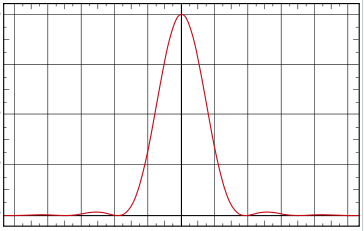 region, the Airy disk, surrounded by concentric bright rings. A graphical representation of an Airy pattern is shown to the right. As a mirror or lens focuses a star, it will appear as an Airy pattern to the observer. In this case the vertical axis represents the intensity of the observed star light and the horizontal axis is a measure of the dimeter of the Airy pattern.

There is a lower limit to the diameter of an Airy disk for a particular mirror or lens. An optical system that has reached this level of perfection is said to be diffraction limited. Reducing system imperfections beyond this point do not reduce the diameter of the Airy disk. The radius of the Airy disk is approximately described by the following equation:

   

where  is the radius of the Airy disk in radians,  is the wavelength of light in meters and  is the diameter of the mirror or lens in meters. Our example telescope (a Celestron CPC 1100 SCT) is diffraction limited and has an aperture of 280mm. In ideal conditions this optical system would produce an Airy disk with a diameter of 0.97” for visible light with a wavelength of 540nm. So an ideal 280mm diffraction limited telescope, without an atmosphere between it and the observed star, would produce an Airy disk with a diameter of 0.97”.

Our atmosphere distorts star light traveling through it. These distortions often occur more than 100 times per second. For long photographic exposures (greater than a few seconds) this movement of the Airy disk results in a larger disk know as a point spread function or seeing disk. This disk is similar in shape to the Airy disk, actually a two-dimensional normal distribution, and its width, generally defined as the full width at half maximum (FWHM), is a measure of the seeing conditions. The best seeing from high altitude mountain observatories is reported to be approximately 0.4”. Most observers seem extremely content with FWHM of 1”, happy with FWHM of 2” and 3” and stop work above 4”. In the next section we’ll use a FWHM equivalent to the diameter of the Airy disk to determine the sensor requirements to accurately represent images captured during perfect observing conditions. If seeing is worse than ideal, the chosen sensor characteristics will be more than adequate.

Sensor and Pixel Size

CMOS sensors are available in a range of sizes with each containing a different number of light collecting elements or pixels. The size of the sensor and the number of pixels determine the pixel size. Sensor size is important because it influences the field of view (FOV) of collected images. Pixel size is important to ensure that the light from each star strikes enough pixels to be sampled properly.

The field of view of a telescope and sensor combination is described by the following equation.

   

where  is the real field of view in radians,  is the size of the sensor in one dimension, measured in meters, and  is the focal length of the optical system also measured in meters. The field of view of a single pixel  is,

   

where  is the size of the sensor in one dimension measured in meters,  is the number of pixels in the same dimension and  is the focal length of the optical system in meters. The ratio of  to  is simply the pixel size, .

   

Nyquist sampling indicates that we need at least two samples of the seeing disk, or the Airy disk in our ideal case, to accurately represent it. Two samples is what is required of one-dimensional signals like audio, but for a two-dimensional system, like the one at hand, it is more like 3.3. In other words,  should be 1/2 to 1/3 the diameter of the Airy disk. We’ll use 1/2 for the remainder of this work which is equal to the Airy disk’s radius.

   

Solving this equation for  and recognizing that  divided by aperture   is equal to the  of the system results in,

   

For an f/2 optical system at 540nm, the ideal pixel size is 1.32µm while the same system operating at f/10 would have an ideal pixel size of 6.59µm. It is unlikely the seeing conditions will ever approach the ideal and will more likely result in FWHM values of between 2” and 4”. At these values the ideal pixel sizes for an f/2 system would be 2.72µm and 5.44µm respectively. For an f/10 system they would be 13.59µm and 27.22µm respectively.

Three commercially available CMOS sensors include the MN34230, IMX294, and the IMX071. These sensors have pixel sizes of 3.8µm, 4.63µm and 4.78µm respectively. These sensor pixels are not quite small enough to offer the ideal sampling at f/2 with good seeing, are satisfactory for imaging in poorer conditions and are more than adequate for imaging at higher f-numbers. In addition, beautiful images can be obtained without reaching these sampling goals, which are often less important for aesthetically pleasing pictures than a large field of view. With a focal length of 560mm these sensors yield fields of view of 1.81°, 1.95° and 2.41° respectively.

Sensor Dynamic Range

Each pixel of a CMOS sensor can only collect so much light energy before it reaches its maximum value or saturation. This point is called full well capacity. When a pixel value is read, it returns the measured intensity of light that struck the pixel and a small error. This read error (and dark current noise) subtracted from the full well capacity represents the dynamic range of the pixel and associated sensor. We’re assuming here that for cooled astrophotography cameras the dark current impact is negligible. This may not be the case, but for comparison purposes it is a reasonable approximation. High dynamic range is a desirable feature.

ADC Capacity

When light strikes a pixel in a CMOS sensor it generates a voltage. This voltage is sampled by an analog to digital converter that translates the voltage into a binary number. The set of binary numbers representing all pixels on the sensor represent the collected image. The number of bits representing each pixel defines how well subtle tonal changes in a scene will be preserved. More bits representing each pixel will result in a final image that is a better representation of the original scene. Typical sensors use 8-14 bits to represent each pixel.

Read Speed

Typically the larger a sensor is in terms of the number of pixels, the slower the read speed. Some sensors permit partitioning allowing portions of the sensor to be read, increasing speed. Read speed is related to frames per second that can be captured. Planetary imaging using lucky imaging techniques require many frames per second. Typical large CMOS sensors have full sensor read speeds between 10 and 30 frames per second. Reduced resolution reads can be done much faster.

Commercially Available Cameras

While there are many commercially available astrophotography cameras from numerous vendors, this document will illustrate just a few. The following table illustrates the specifications for cameras based on the MN34230, IMX294, and IMX071 CMOS sensors. Two of the cameras are based on the same sensor, but have slightly different specifications. In the next section we’ll consider which characteristic of each camera is a best match for our application.

	ASI1600MC Pro	ASI294MC Pro	ASI071MC Pro	QHY168C
Cost	$999	$1080	$1680	$1499
Resolution	16MP 4656 x 3520	11.3MP 4144 x 2822	16MP 4944 x 3284	16MP 4952 x 3288
Pixel Size	3.8µm	4.63µm	4.78µm	4.78µm
Sensor	MN34230	IMX294	IMX071	IMX071
Sensor Size	17.7 x 13.4mm	19.1 x 13mm	23.6 x 15.6mm	23.6 x 15.6mm
Sensor Diagonal	22.2mm	23.2mm	28.4mm	28.4mm
Capture Speed	23 FPS	19 FPS	10 FPS	10 FPS
Read Noise	1.2 - 3.6e	1.2 - 7.3e	2.3 - 3.3e	2.3 - 3.3e
Full Well Capacity	20000e	63700e	46000e	46000e
Dynamic Range (no dark current)	75 db	79 db	83 db	83 db
ADC	12 bits	14 bits	14 bits	14 bits
Cooling	40°-45°	35°	35°-40°	35°
Memory Buffer	256MB DDRIII	256MB DDRIII	256MB DDRIII	128MB DDRII
FOV @ 560mm FL	1.81° x 1.37°	1.95° x 1.33°	2.41° x 1.6°	2.41° x 1.6°
FOV per Pixel @ 560mm FL	1.4"	1.69"	1.75"	1.75"
Diameter	78mm	78mm	86mm	90mm

Our Application

In this section we’ll consider each CMOS camera illustrated in the previous table and how it fits our application. We desire a camera that will be useful for DSO imaging in conjunction with a Fastar or Hyperstar system connected to a CPC 1100 GPS XLT telescope. We would also like to use the same camera for planetary imaging connected to the same telescope in its f/10 configuration augmented with Barlow lenses to increase the f-number to f/20 or f/30.

Form Factor

Each of the four cameras are cylindrical in shape with diameters that are less than the diameter of the secondary mirror of the Celestron CPC 1100 telescope. In other words, none of the cameras obstruct the useful aperture and all have the same cabling, causing unwanted diffraction. These cameras will also connect fine in the f/10 configuration.

Sensor and Pixel Size

In the f/2 configuration, with perfect seeing, we could use a pixel size of 1.32µm, but with realistic expectations of FWHM of 3”, Nyquist requires a pixel size of 4.08µm. Only the ASI1600MC Pro has a pixel size that meets this requirement. In the f/10 configuration, all of the cameras meet Nyquist’s requirement. In fact, the large pixel size of the two cameras using the IMX071 sensor would meet the sampling requirement down to f/7, using a focal reducer, with perfect conditions, and lower under realistic seeing.

Dynamic Range and ADC

The larger pixels of the ASI294MC Pro, ASI071MC Pro and the QHY168C result in higher full well capacities that in turn result in potentially better dynamic range. This is particularly important when operating at f/2 when bright stars within the large field of view may quickly saturate some pixels. In addition, these three cameras also have 14 bit ADCs that may result in slightly more accurate images.

Read Speed

The four cameras range in speed from a low of 10 fps to a high of 23 fps. However, each is capable of higher speeds at lower resolutions. For example, the QHY168C is capable of frame rates as high as 130 fps for 240 lines of resolution and 30 fps for 1920 x 1080 HD. These rates should be adequate for useful planetary imaging in good seeing conditions.

Best Fit

In this section we’ll refer to data in the above table and point out meaningful characteristics that are best met by the associated camera. The camera with the best pixel size that approaches proper sampling is the ASI1600MC Pro. However, none of the cameras have small enough pixels to meet the demands of Nyquist’s sampling requirements for ideal seeing conditions. As previously stated, beautiful images can be obtained without reaching the Nyquist sampling goals and these goals are often less important than obtaining a large field of view.

Since the field of view is directly related to the sensor size, the ASI071MC Pro and the QHY168C are the big winners. Their fields of view are nearly 1/2° wider than the next best camera. In addition, these two cameras have better dynamic range and have the same size ADCs.

In comparing the ASI071MC Pro and the QHY168C, the ASI071MC Pro has a larger memory buffer made of DDRIII instead of DDRII memory. It also achieves a slightly cooler temperature which should further increase its dynamic range beyond that of the QHY168C. The ASI071MC Pro includes a 2-port USB 2.0 hub, is 60g lighter and insignificantly smaller. Finally, the QHY168C is currently $181 less expensive than the ASI071MC Pro.

The following table illustrates the components that are necessary to use the Celestron CPC 1100 GPS XLT telescope for astrophotography. Note that the additional $181 for the ASI071MC Pro adds only 5% to the total cost of the project. This seems reasonable given the slight feature advantages it has over its competitor.

	ASI071MC Pro	QHY168C
Celestron HD Wedge	$350	$350
Camera	$1680	$1499
Hyperstar 3	$999	$999
10:1 Focuser	$275	$275
Bahtinov Mask	$35	$35
Total	$3339	$3158

Summary

The convertible feature of the Celestron CPC 1100 GPS XLT telescope makes the system useful for imaging planets in its f/10 configuration, while its f/2 configuration, using Fastar or Hyperstar, yields a massive 2.7° field of view for imaging DSOs. While none of the reviewed cameras have small enough pixels to satisfy Nyquist sampling requirements for theoretical seeing conditions in the f/2 configuration, two of the four are adequate and yield 2.4° fields of view. For planetary imaging these two cameras easily meet the sampling requirements and have fast enough frame rates to support lucky imaging techniques. While the cost of the ASI071MC Pro is slightly higher than the QHY168C, the ASI071MC Pro reaches cooler temperatures, has a USB hub that may reduce wiring congestion, is 60g lighter and is slightly smaller. Overall, the ASI071MC Pro is our best fit.